Percentage

Calculating percentages in Excel is easy. Percentage simply means 'out of 100', so 72% is '72 out of 100' and 4% is '4 out of 100', etc.

Enter a Percentage

To enter a percentage in Excel, execute the following steps.

First, enter a decimal number.

On the Home tab, in the Number group, click the percentage symbol to apply a Percentage format.

Here the result.

Note: To change the percentage in cell A1, simply select cell A1 and type a new percentage (do not type a decimal number). 

Percentage of Total

To calculate the percentage of a total in Excel, execute the following steps.

First, enter the formula is shown below. This formula divides the value in cell A1 by the value in cell B1. Simply use the forward slash (/) as the division operator. Don't forget, always start a formula with an equal sign (=).

On the Home tab, in the Number group, click the percentage symbol to apply a Percentage format.

Here the result.

On the Home tab, in the Number group, click the Increase Decimal button once.

Here the result of percentage with one decimal place.

Note: Excel always uses the underlying precise value in calculations, regardless of how many decimals you choose to display.

Increase by Percentage

To increase a number by a percentage in Excel, execute the following steps.

First, enter a number in cell A1. Enter a decimal number (0.2) in cell B1 and apply a Percentage format.

To increase the number in cell A1 by 20%, multiply the number by 1.2 (1+0.2). The formula below does the trick.

To decrease a number by a percentage, simply change the plus sign to a minus sign.

Note: Excel uses a default order in which calculations occur. If a part of the formula is in parentheses, that part will be calculated first.

Percentage Change

To calculate the percentage change between two numbers in Excel, execute the following steps.

Enter an old number in cell A1 and a new number in cell B1.

First, calculate the difference between new and old.

Next, divide this result by the old number in cell A1.

On the Home tab, in the Number group, click the percentage symbol to apply a Percentage format.

Here the result.

The (New-Old)/Old formula always works.

Note: Excel uses a default order in which calculations occur. If a part of the formula is in parentheses, that part will be calculated first.

Multiply

To multiply numbers in Excel, use the asterisk symbol (*) or the PRODUCT function. Learn how to multiply columns and how to multiply a column by a constant.

• The formula below multiplies numbers in a cell. Simply use the asterisk symbol (*) as the multiplication operator. Don't forget, always start a formula with an equal sign (=).

• The formula below multiplies the values in cells A1, A2 and A3.

• As you can imagine, this formula can get quite long. Use the PRODUCT function to shorten your formula. For example, the PRODUCT function below multiplies the values in the range A1: A7.

• Here's another example.
  

Explanation: =A1*A2*A3*A4*A5*A6*A7*B1*B2*B3*B4*C1*8 produces the exact same result.

 To multiply two columns, execute the following steps.

First, multiply the value in cell A1 by the value in cell B1.

Next, select cell C1, click on the lower right corner of cell C1 and drag it down to cell C6.

To multiply a column of numbers by a constant number, execute the following steps.

First, multiply the value in cell A1 by the value in cell A8. Fix the reference to cell A8 by placing a $ symbol in front of the column letter and row number ($A$8).

 Next, select cell B1, click on the lower right corner of cell B1 and drag it down to cell B6.

Explanation: when we drag the formula down, the absolute reference ($A$8) stays the same, while the relative reference (A1) changes to A2, A3, A4, etc. You can also use Paste Special to quickly multiply a range of cells by a constant number.

Enter a formula

A formula is an expression which calculates the value of a cell. Functions are predefined formulas and are already available in Excel.

To enter a formula, execute the following steps.

1. Select a cell. 
2. To let Excel know that you want to enter a formula, type an equal sign (=). 
3. For example, type the formula A1+A2.  
   
4. Change the value of cell A1 to 3.
   

Tip: instead of typing A1 and A2, simply select cell A1 and cell A2.

Subtract

There's no SUBTRACT function in Excel. However, there are several ways to subtract numbers in Excel. Are you ready to improve your Excel skills?

• For example, the formula below subtracts numbers in a cell. Simply use the minus sign (-). Don't forget, always start a formula with an equal sign (=).

• The formula below subtracts the value in cell A2 and the value in cell A3 from the value in cell A1. 
  

• As you can imagine, this formula can get quite long. Simply use the SUM function to shorten your formula. For example, the formula below subtracts the values in the range A2: A9 from the value in cell A1.
  

To subtract the numbers in column B from the numbers in column A, execute the following steps.

• First, subtract the value in cell B1 from the value in cell A1.
  
• Next, select cell C1, click on the lower right corner of cell C1 and drag it down to cell C6.
  

To subtract a number from a range of cells, execute the following steps. 

1. First, subtract the value in cell A8 from the value in cell A1. Fix the reference to cell A8 by placing a $ symbol in front of the column letter and row number ($A$8).
   
2. Next, select cell B1, click on the lower right corner of cell B1 and drag it down to cell B6.
   

When we drag the formula down, the absolute reference ($A$8) stays the same, while the relative reference (A1) changes to A2, A3, A4, etc. Maybe this is one step too far for you at this stage, but it shows you one of the many other powerful features Excel has to offer.

Printing your Workbook

Print Commands

In Office, you can print and preview files from the same location by clicking File and then Print.

Print Preview

Excel combines Print and Preview in the same window.

1. Click File > Print. On the right, you’ll see a preview of your file. On the left, you'll see the Print button and the configurable Settings. 
2. Choose the number of copies you want. 
3. Look under Settings to choose other print options such as printing only certain pages, changing the page orientation, or printing two-sided. 
4. When you are ready, click Print. 
5. Click the arrow to return to your document.

Using Basic Print Options

Basic print options are available next to the preview.

• Print settings can also be found from the Page Layout tab.

Other Print Options

To access to more options, click on Page Setup on the bottom-right corner of the basic print options or by clicking on the dialog box launchers on the bottom-right corner of Page Setup, Scale to Fit and Sheet Options group in the Page Layout tab.

Using the View Tab

Excel offers three workbooks views, Normal, Page Layout and Page Break Preview.

Using Normal View

1. On the View tab, in the Workbook Views group, click Normal.

Note: if you switch to another view and return to Normal view, Excel displays page breaks. Close and reopen the Excel file to hide these page breaks. To always hide page breaks for this worksheet, click File, Options, Advanced, scroll down to Display options for this worksheet and uncheck Show page breaks. 

Using Full Screen View

To view more data on the screen, you can temporarily switch to full-screen view. Full-screen view hides the Microsoft Office Fluent user interface Ribbon, the formula bar, and the status bar. To have access to the hidden elements again, you have to return to normal screen view.

• To switch to the full-screen view, on the View tab, in the Workbook Views group, click Full Screen. 
• To return to normal screen view, right-click anywhere in the worksheet, and then click Close Full Screen or press ESC in the keyboard.

Note: The Full-screen option is not available in Excel 2013 and later versions. However, you can always hide the ribbon, tabs, or commands, to maximize the screen space in Excel.  

Using Page Layout View

Use Page Layout view to see where pages begin and end, and to add headers and footers.

1. On the View tab, in the Workbook Views group, click Page Layout.

Page Break Preview

Page Break Preview gives you a nice overview of where pages break when you print the document. Use this view to easily click and drag page breaks.

1. On the View tab, in the Workbook Views group, click Page Break Preview.
   

Note: 

• Click and drag the page breaks to fit all the information on one page. Be careful, Excel doesn't warn you when your printout becomes unreadable. 
• By default, Excel prints down, then over. In other words, it prints all the rows for the first set of columns. 
• Next, it prints all the rows for the next set of columns, etc. (take a look at the page numbers in the picture above to get the idea). 
• To switch to Print over, then down, click File, Print, Page Setup, on the Sheet tab, under Page order, click Over, then down. 

Working with Charts, Part 1

Creating a Chart

You can create a basic chart by selecting any part of the range you want to be charted, then clicking the chart type that you want on the Insert tab in the Charts ribbon group. Or, simply press Alt+F1 for Excel to automatically create a simple column chart for you. From there, you have multiple options to change the chart so it's just the way you want it.

Inserting a Column Chart

1. Select the data from the spreadsheet.
2. Click Insert > Insert Column or Bar Chart icon, and select a column chart option of your choice. 
   

Inserting a Line Chart 

1. Select the data from the spreadsheet. 
2. Click Insert > Insert Line or Area Chart icon, and select a chart option of your choice.

Inserting a Bar Chart 

1. Select the data from the spreadsheet. 
2. Click Insert > Insert Column or Bar Chart icon, and select a chart option of your choice.

Inserting a Pie Chart

1. In your spreadsheet, select the data to use for your pie chart. 
2. Click Insert > Insert Pie or Doughnut Chart, and then pick the chart you want.

Styling Charts with the Design Tab

1. Click the chart that you want to format. This displays the Chart Tools, adding the Design, Layout, and Format tabs.
2. On the Design tab, in the Chart Styles group, click the chart style that you want to use.
   

Tip: To see all predefined chart styles, click More.

Notes:
• When the Excel window is reduced in size, chart styles will be available in the Chart Quick Styles gallery in the Chart Styles group.
• Chart styles use the colors of the current document theme that is applied to the workbook. You can change the colors by switching to a different document theme. You can also customize a document theme to display a chart in the exact colors that you want.

Modifying Charts with the Layout Tab

After you create a chart, you can instantly change its look. Instead of manually adding or changing chart elements or formatting the chart, you can quickly apply a predefined layout and style to your chart. 

Microsoft Office provides a variety of useful predefined layouts and styles (or quick layouts and quick styles) that you can select from. However, you can customize a layout or style of a chart further by manually changing the layout and style of the individual chart elements that are used in the chart.

Select a predefined chart layout

1. Click the chart that you want to format. This displays the Chart Tools, adding the Design, Layout, and Format tabs. 
2. On the Design tab, in the Chart Layouts group, click the chart layout that you want to use.

Manipulating a Chart

You can change the format of individual chart elements, such as the chart area, plot area, data series, axes, titles, data labels, or legend.

1. Select the chart element (for example, data series, axes, or titles), right-click it, and click Format <chart element>. 
2. The Format pane appears with options that are tailored for the selected chart element.
3. Clicking the small icons at the top of the pane moves you to other parts of the pane with more options. 
4. If you click on a different chart element, you’ll see that the task pane automatically updates to the new chart element.

Enhancing a Worksheet’s Appearance

Adding Patterns and Colors

Formatting the Background Color

You can highlight data in cells by using Fill Color to add or change the background color or pattern of cells. Here's how;

1. Select the cells you want to highlight. 
2. Click Home > the arrow next to Fill Color, or press Alt+H, H. Under Theme Colors or Standard Colors, pick the color you want. 
3. To use a custom color, click More Colors, and then in the Colors dialog box select the color you want.
   

Tip: 

• To use a different background color for the whole worksheet, click the Select All button. This will hide the grid lines, but you can improve worksheet readability by displaying cell borders around all cells.
• To applies the most recently selected color, you can just click Fill Color. You'll also find up to 10 most recently selected custom colors under Recent Colors.

Apply a pattern or fill effects

When you want something more than a just a solid color fill, try applying a pattern or fill effects.

1. Select the cell or range of cells you want to format. 
2. Click Home > Format Cells dialog launcher, or press Ctrl+Shift+F. 
3. On the Fill tab, under Background Color, pick the color you want.
   

Adding Borders

To apply a new or different border style, click the arrow next to Borders, and then click a border style.

1. To apply a custom border style or a diagonal border, click More Borders. 
2. In the Format Cells dialog box, on the Border tab, under Line and Color, click the line style and color that you want. 
3. Under Presets and Border, click one or more buttons to indicate the border placement. Two diagonal border buttons are available under Border.

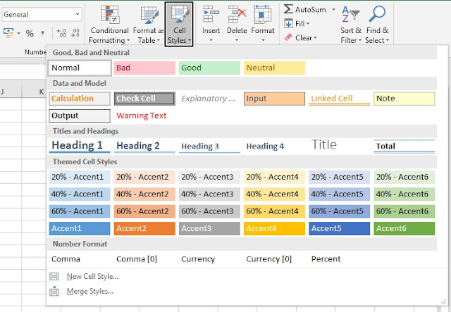
Working with Styles

Microsoft Office Excel has several built-in cell styles that you can apply or modify. You can also modify or duplicate a cell style to create your own, custom cell style.

1. Select the cells that you want to format. 
2. On the Home tab, in the Styles group, click the More drop-down arrow in the style gallery, and select the cell style that you want to apply.

Important: Cell styles are based on the document theme that is applied to the whole workbook. When you switch to another document theme, the cell styles are updated to match the new document theme.

Working with Themes

Themes make it easy to coordinate colors, fonts, and graphic formatting effects across your Word, Excel, and PowerPoint documents and update them quickly. You can change the entire theme or just customize theme fonts, colors, or effects. 

• To change themes, simply pick a different theme from the Themes menu. 
• To return to the default theme, choose the Office theme. 
• To remove theme formatting from just a portion of your document, select the portion you want to change and change any formatting you like, such as font style, font size, color, etc.

Anything you can do to enhancing appearance in Excel. So that your data will be more neat.

Cell Formatting

Cell Formatting in Excel

The Format Painter

The format painter lets you copy all formatting from one object and apply it to another one.

1. Select the text or graphic that has the formatting that you want to copy. 
2. On the Home tab, click Format Painter. The pointer changes to a paintbrush icon. 
3. Use the brush to paint over a selection of text or graphics to apply the formatting. This only works once. 
4. To change the format of multiple selections in your document, you must first double-click Format Painter. 
5. Then to stop formatting, press ESC.

Note: If you want to copy text formatting, select a portion of a paragraph. If you want to copy text and paragraph formatting, select an entire paragraph, including the paragraph mark.  

Cell Merging and AutoFit

Cell Merging

There are a few cells merging;

1. Combine and center the content of selected cells in a new larger cell. This is a great way to create a label that spans multiple columns.
   
2. Merge selected cells in the same row into one large cell. 
   
3. Merge selected cells into one cell.
   

AutoFit

AutoFit will enable you to resize and adjust height and width rows and columns instantly. Learn the exact steps on how to apply to autofit in your Excel-spreadsheet.

1. Select the columns or rows that you want to change. 
2. On the Home tab, in the Cells group, click Format. 
3. Under Cell Size, click AutoFit Column Width or AutoFit Row Height.